3D Reconstruction from Satellite Imagery

Jeremy Fischer, Jakob Gollreiter, Daniel Won

Code: https://github.com/JakobMichaelGollreiter/3d-gaussian-splatting-satellite-images

Abstract: We investigate the feasibility of 3D reconstruction from limited and variable-quality satellite imagery (10-20 views per scene). Through comparison of three approaches - 3D Gaussian Splatting with derived camera parameters, VGGT followed by bundle adjustment, and DUSt3R - we demonstrate that practical 3D reconstruction is achievable despite challenging input conditions. Our evaluation shows VGGT with bundle adjustment produces the most geometrically accurate results, while optimized DUSt3R offers the most reliable reconstructions.

1. Introduction

Computer vision problems such as segmentation and classification have been the core focus of satellite image processing research, but 2D-to-3D reconstruction is a novel subtopic that has yet to be fully explored. Current systems such as Google Earth are capable of creating 3D representations of urban geometry, but these may require more sophisticated technology such as LiDAR, a large image dataset, and additional expenses to collect sufficient data. However, applications such as analyzing geographic impacts of natural disasters require efficient, quick data collection and results, which may not be possible with typical reconstruction methods.

We aim to explore whether meaningful 3D structure can be reconstructed from sparse satellite imagery, where each scene includes only 10 to 20 top-down views with varying lighting and quality. As methods such as neural radiance fields (NeRFs) are computationally expensive, we have explored alternatives that exhibit faster training times and/or are capable of extracting sufficient visual data from sparse image sets.

2. Dataset

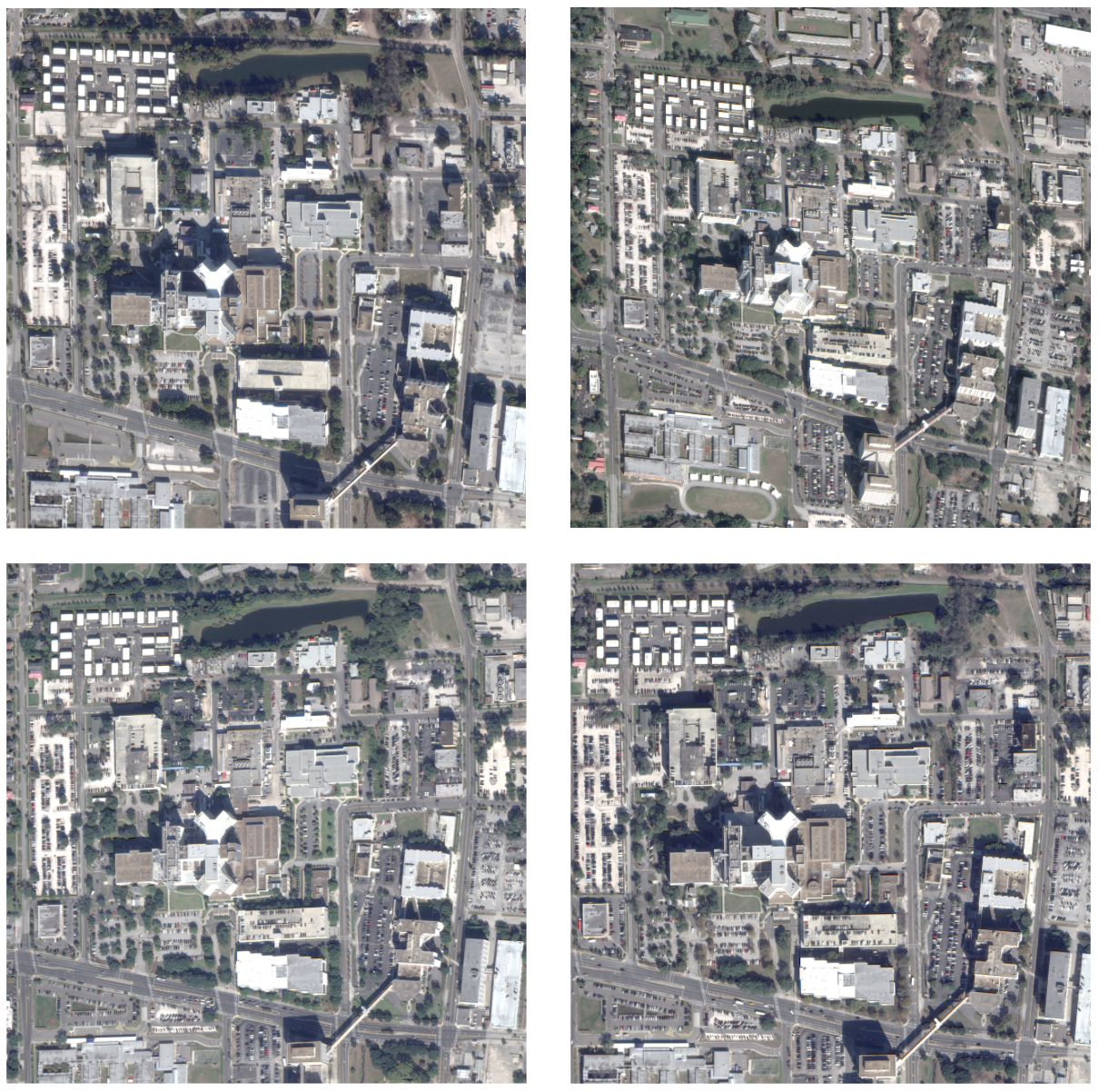
For our project we use Track 3 of the 2019 IEEE GRSS Data Fusion Contest (DFC2019), which comprises 110 scenes with approximately 20 multi-angle satellite images per scene (about 2,200 images total). Each scene includes multiple perspective views captured from slightly different angles (see Figure below), providing the multi-view geometry necessary for 3D reconstruction.

Figure 1: Four different satellite views from a scene of the DFC2019 dataset

3. Related Works

Preliminary investigations used NeRFs for satellite image reconstructions as "digital surface models". Marí et al. introduced methods of "Sat-NeRFs" and "Earth Observation NeRFs" (EO-NeRFs) that apply shadow modeling to extract color and height data. However, expensive runtime can be critical drawbacks for these solutions' applicability of these NeRF solutions. Studies such as Billouard et al.'s SAT-NGP method aim to develop faster methods via graphics primitives to reduce 20 hours of computation time to roughly 13 to 14 minutes, although there is reportedly some loss in output quality.

Recent studies investigated 3D Gaussian splatting (3DGS) as a faster, more efficient alternative to NeRF methods while employing similar methods. Gao et al. applied the original 3DGS method on urban scenes captured in Google Earth datasets, although these images tend to include a variety of 3D viewpoints that cover multiple perspectives, angles, and altitudes to extract more accurate 3D geometry. Aira et al. introduced "Earth Observation Gaussian Splatting" (EOGS) which integrates the shadow model from NeRF methods with 3DGS and 3 additional regularizations for sparsity, view consistency, and opaqueness, resulting in a runtime of about 3 minutes (about 8 times faster than SAT-NGP and 300 times faster than EO-NeRF). EOGS is a promising start to extracting geometric information from 2D satellite images, but it is limited in that it focuses more on generating depth maps than on a full 3D reconstruction.

4. Methodology

In this section, we describe our approach to 3D reconstruction from satellite imagery. We first extract camera parameters from satellite metadata and approximate camera extrinsics, followed by a view selection process that identifies the optimal images. We then implement and evaluate three different reconstruction methods: 3D Gaussian Splatting (3DGS), Visual Geometry Grounding Transformer (VGGT) with bundle adjustment optimization, and DUSt3R.

4.1 Camera Extrinsics Approximation

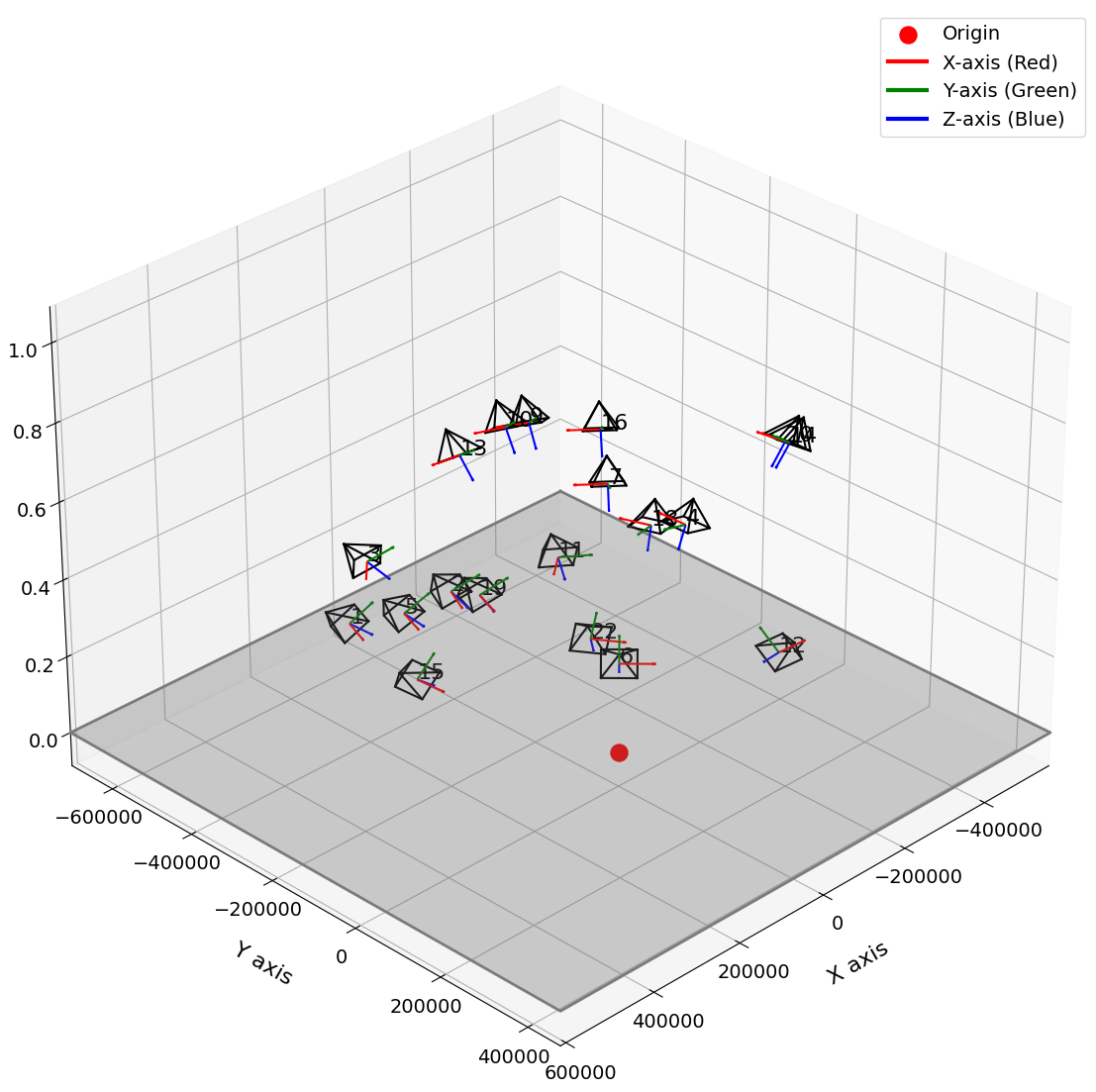
Our dataset includes Rational Polynomial Coefficients (RPCs) embedded in TIFF files as metadata for each scene view. We derive approximate physical camera parameters from these RPCs (see Figure below). Though not exact, our camera extrinsic approximations preserve the essential geometric relationships between views, which is sufficient for optimal image selection in our reconstruction pipeline.

4.1.1 Rational Polynomial Coefficients

Rational Polynomial Coefficients are a mathematical model used in satellite imagery to establish the geometric relationship between the image coordinates (row, column) and the corresponding ground coordinates (latitude, longitude, height). They map between the 2D image space and 3D world space without needing to know the exact physical sensor model.

4.1.2 Rotation Matrix Derivation

We derive camera rotation by analyzing height-sensitive RPC coefficients that encode how image coordinates change with elevation. These coefficients correlate with viewing angles, allowing us to estimate the satellite's off-nadir angle (tilt from vertical) and azimuth angle (compass direction). Off-nadir angle is calculated from the height coefficient gradient's magnitude, while azimuth is determined from how height changes affect line and sample coordinates.

4.1.3 Translation Vector Derivation

Using the estimated off-nadir and azimuth angles, we calculate satellite position relative to the ground point using spherical coordinate principles, with distance based on orbital height and viewing angle. Ground points are converted from geographic coordinates to a local East-North-Up coordinate system with a central reference point.

Visualization of relative satellite camera positions with respect to fix point — Figure 2: Visualization of relative satellite camera positions with respect to fixed point

4.2 Camera Spread and Selection

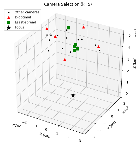
Some training methods, such as Dust3R, exhibit exponential increases in train time as the number of training images grows, making wise image selection critical. We additionally hypothesize that output quality depends on the spatial distribution of camera viewpoints, since a wider range provides more representative coverage of different perspectives. To investigate this, we apply Fisher information theory to identify subsets of images that maximize and minimize camera spread based on their extrinsic parameters. Since all images share the same focus point, we quantify the spread solely in terms of relative longitude, latitude, and altitude.

Specifically, we first compute the unit viewing direction \(\mathbf{u}_i\in\mathbb{R}^3\) for each camera \(i\) by normalizing its offset from the focus point:

\(\mathbf{u}_i = -\frac{\mathbf{p}_i - \mathbf{f}}{\|\mathbf{p}_i - \mathbf{f}\|}\)

where \(\mathbf{p}_i\) and \(\mathbf{f}\) denote the \(i\)th camera position and the focus point.

Given any subset \(S\) of size \(k\), we form the Fisher information matrix:

\(\mathbf{F}_S = \sum_{i\in S} \mathbf{u}_i\,\mathbf{u}_i^\top\)

whose determinant \(\det(\mathbf{F}_S)\) quantifies the volumetric spread of those views.

To approximate the D-optimal subset, we use the following greedy procedure:

Initialize \(S \leftarrow \emptyset\).
Repeat until \(|S| = k\):
1. For each candidate \(j \notin S\), compute \(\displaystyle \Delta_j = \det\Bigl(\sum_{i\in S\cup\{j\}}\mathbf{u}_i\,\mathbf{u}_i^\top\Bigr).\)
2. Select \(j^* = \arg\max_{j\notin S} \Delta_j\) and update \(S \leftarrow S \cup \{j^*\}.\)

This avoids the combinatorial cost of brute-force search while providing an efficient \(O(n\,k\,d^3)\) approximation to the true D-optimal selection.

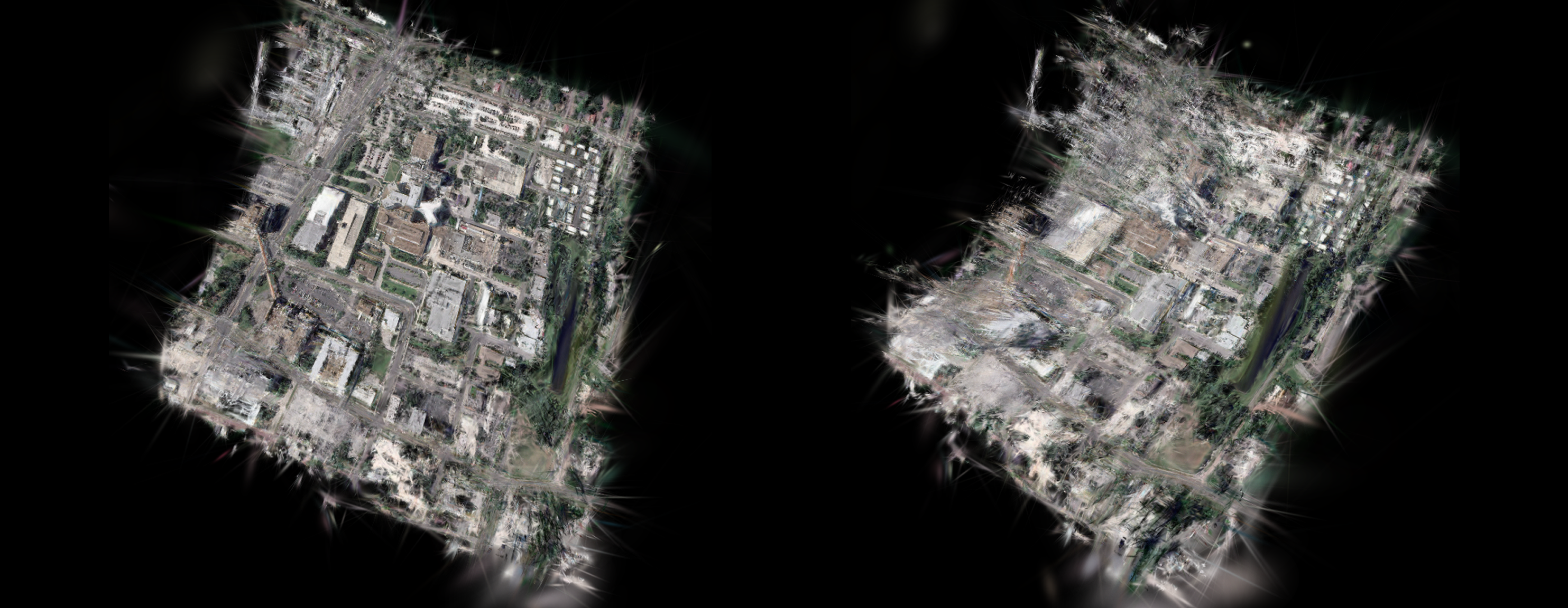
Figure 3: Visualization of most and least camera spread from greedy algorithm. Least-spread could roughly lie on a plane providing no views perpendicular to the left and right.

4.3 3D Gaussian Splatting (3DGS)

3D Gaussian splatting represents scenes via Gaussian ellipsoids that we train and optimize. The scene is initialized as a point cloud where each Gaussian point has properties such as position, shape, color, and opacity that are updated to minimize the photometric reconstruction loss.

The original 3DGS codebase takes in two types of data structures: (1) COLMAP representations, which contain binary or text files of camera extrinsics, camera intrinsics (including field of view), and initial 2D-to-3D point correspondences, and (2) transform JSON files used for NeRFs that only contain information about the extrinsics and intrinsics. While both data structures can theoretically be used for training, the COLMAP structure appears to be most supported by 3DGS as it carries more metadata such as initial point correspondences for facilitating point cloud optimizations.

4.3.1 Data Preparation

Using 3DGS's convert.py function, we ran SfM via COLMAP on our dataset, extracting the initial point cloud and camera parameters from satellite images into a COLMAP data structure. For 3DGS, we use the pinhole camera model in which our core intrinsics are the focal lengths f_x, f_y and the optical centers c_x, c_y, which we assume to be (S/2, S/2) for the square image dimension of S × S. (For our data, S = 2048 pixels, so our optical center is (1024, 1024)). We also used Depth Anything V2 to extract initial depth maps for the scene to contribute to depth regularization for a more accurate topology.

Figure 4: Generated depth maps from Depth Anything V2 with brighter spots reflecting taller geometry

4.3.2 Results

Our results show that of 16 views, only 3 contained point correspondences were consistently detectable by COLMAP. For 3 images, training took about 11 minutes for 10,000 iterations on an NVIDIA Tesla T4 GPU using Google Colab Pro. Without depth regularization, we achieved a final training L1 loss of 0.0195 and a PSNR of 35.61 and with depth regularization, loss and PSNR stayed relatively the same at around 0.0196 and PSNR of 35.59 with similar rendered results. With only a few input images with small variations in viewpoints and similar camera properties, 3DGS and COLMAP are unable to extract enough meaningful features about the world geometry. Our results imply that simply using the vanilla 3DGS approach may not be sufficient for our sparse image dataset.

Figure 5: Rendered results of 3DGS: the left image shows the ideal view where it appears the closest to the ground truth, and the right image shows a different view visualizing significant artifacts

4.4 VGGT + Bundle Adjustment

Our second approach combines VGGT with classical bundle adjustment optimization. We use VGGT for the initial camera parameters and the 3D point cloud estimates, then apply specialized bundle adjustment for refinement.

4.4.1 VGGT Foundation

The Visual Geometry Grounding Transformer (VGGT) processes multi-view images through a streamlined architecture using DINO-based patch extraction and alternating attention between within-frame and cross-frame relationships. In a single forward pass, VGGT outputs camera parameters, per-pixel depth maps with confidence scores, and world-space 3D coordinates.

4.4.2 VGGT + Bundle Adjustment

Our bundle adjustment implementation jointly optimizes camera poses and 3D point positions to minimize reprojection loss, with these key components:

Confidence-Based Point Selection: We use VGGT's per-pixel confidence scores to filter unreliable 3D points. For selected points, we store 2D image coordinates, 3D world coordinates, and camera indices, establishing global constraints for optimization.
Differentiable Reprojection Model: Our differentiable reprojection function uses the pinhole camera model to project 3D points into 2D image coordinates through extrinsic parameters (R, t), normalized coordinates, and intrinsic camera matrix (K). This enables gradient-based optimization while tracking point depths.
Loss Functions: We implement Huber loss for outlier robustness by transitioning from quadratic to linear behavior beyond a threshold, orthogonality loss to maintain valid rotation matrices (\(R \cdot R^\top = I\)) preserving geometric integrity, and depth penalty to enforce physical plausibility by penalizing negative depths. This combined approach ensures optimization remains mathematically sound and physically valid.
\(\mathcal{L} = \mathcal{L}_{\text{reproj}} + \mathcal{L}_{\text{depth}} + \mathcal{L}_{\text{ortho}}\)

\(\mathcal{L}_{\text{ortho}} = \frac{1}{S} \sum_{j=1}^{S} \|\mathbf{R}_j \mathbf{R}_j^T - \mathbf{I}_3\|_F^2\)
Multi-Stage Optimization: We implement a progressive optimization approach starting with only the highest-confidence points to establish accurate camera positions, then gradually incorporating lower-confidence points in subsequent stages. This prevents less reliable points from disrupting initial structural estimation while still utilizing them for enhanced detail in later stages.

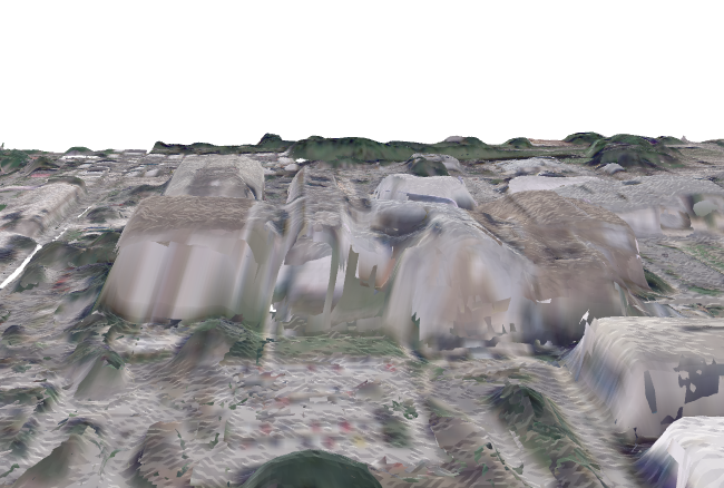
4.4.3 Results

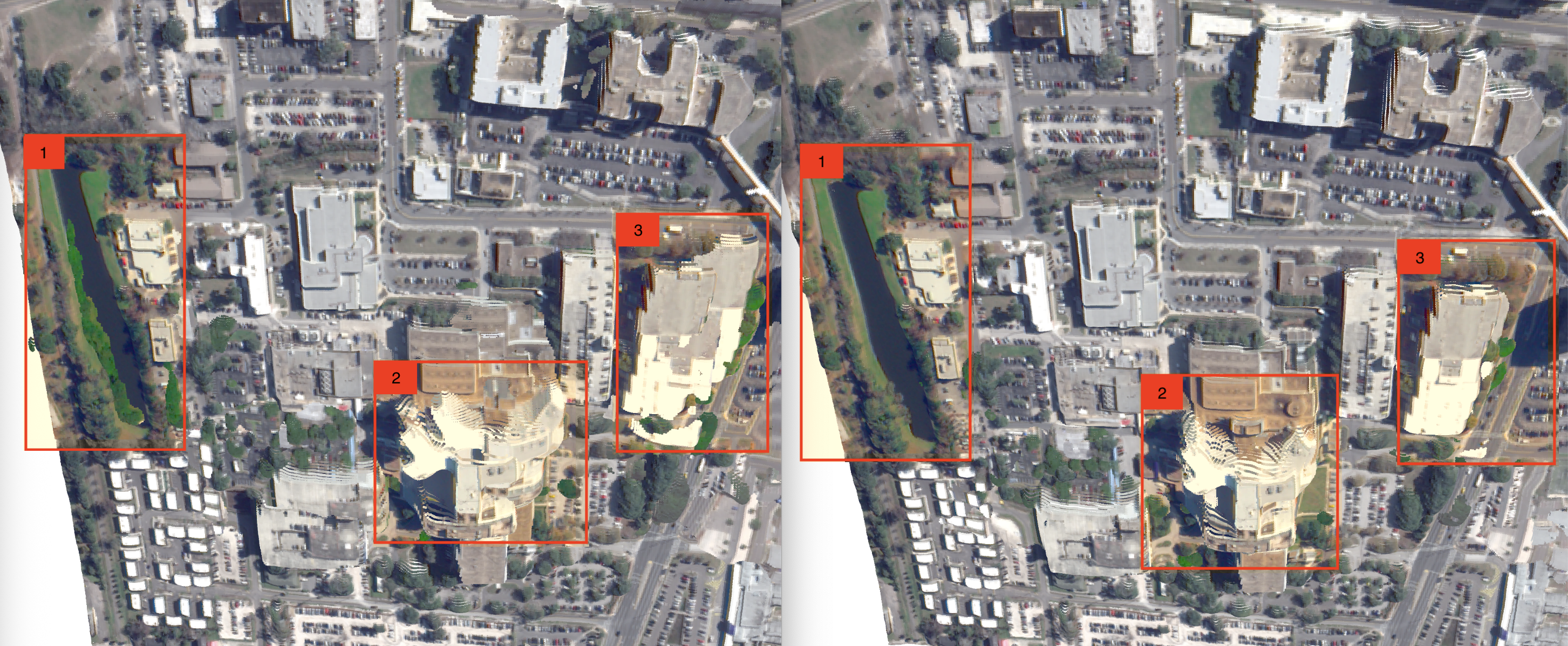
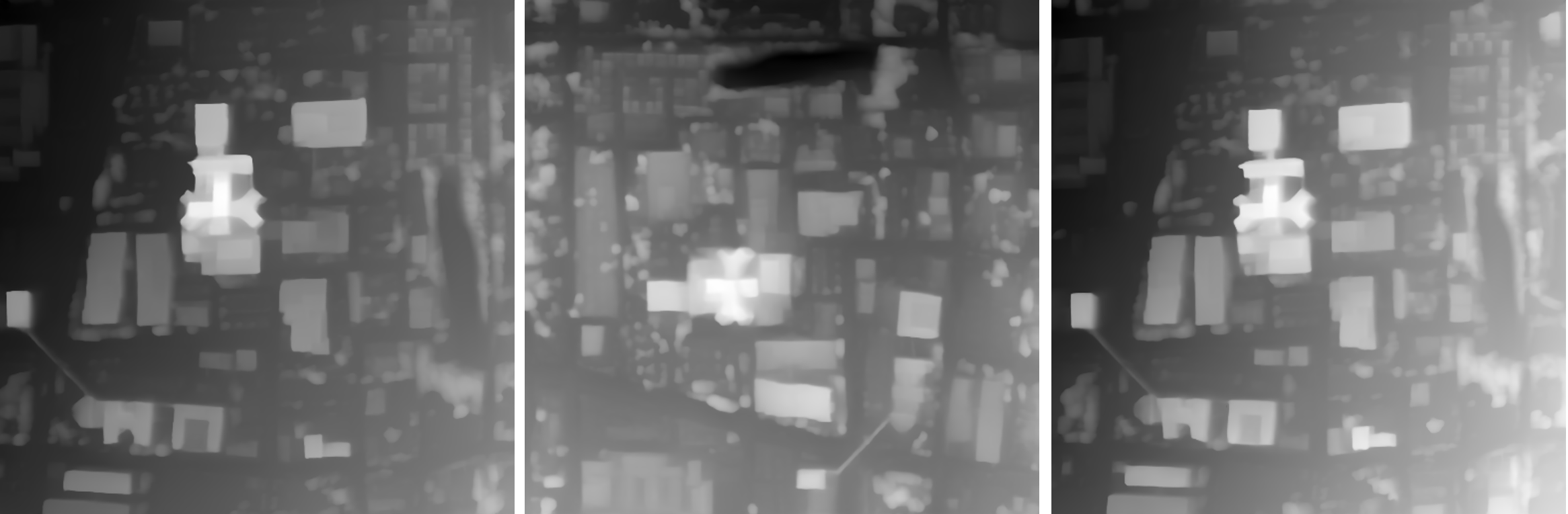
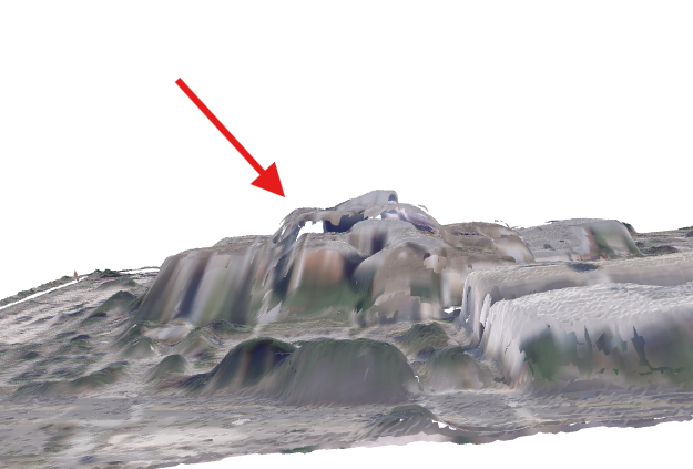
Visualization of VGGT and VGGT + Bundle Adjustment — Figure 6: Visualization of VGGT (left) and VGGT + Bundle Adjustment (right). Red boxes highlight three key improvements: (1) elimination of artifacts in surfaces, (2) enhanced definition of tall buildings with reduced distortion, and (3) improved geometric coherence across boundaries.

For this experiment, we used 4 views from the scene selected using the maximum camera spread criteria. VGGT already performs a good general reconstruction. The subsequent bundle adjustment yields significant improvements, particularly evident in three highlighted areas:

Surface Correction: Bundle adjustment successfully removes artifacts, creating clean, physically plausible surfaces.
Building Definition: Complex vertical structures show reduced distortion, with sharper edges and better preservation of geometry.
Global Coherence: The refined model exhibits improved alignment between scene elements, with fewer inconsistencies at structural boundaries.

4.5 DUSt3R

DUSt3R is a neural network approach for 3D reconstruction that creates consistent three-dimensional models from collections of uncalibrated images without known camera positions. It works by generating dense pointmaps, which map pixels to 3D coordinates. The system uses a transformer architecture with a shared encoder and cross-attention decoders to process image pairs and produce pointmaps in a common reference frame. From these pointmaps, the system can determine camera parameters, pixel correspondences, depth information, and camera poses.

4.5.1 DUSt3R + View Selection

DUSt3R suffers from a combinatorial explosion in training time as additional images are included due to its cross-referencing mechanism. Although DUSt3R learns extrinsics and cannot be directly inserted, we hypothesized that we could achieve better quality output by using our position extractions and a greedy algorithm to find the optimal views. Additionally, this would solve the infeasibility of training on the entire image group.

Number of Images	Time (s)
2	6
4	24
8	58
16	6152

Table 1: Training time (in seconds) measured on a system with 32 GB RAM and an NVIDIA RTX 3060 GPU.

4.5.2 Results

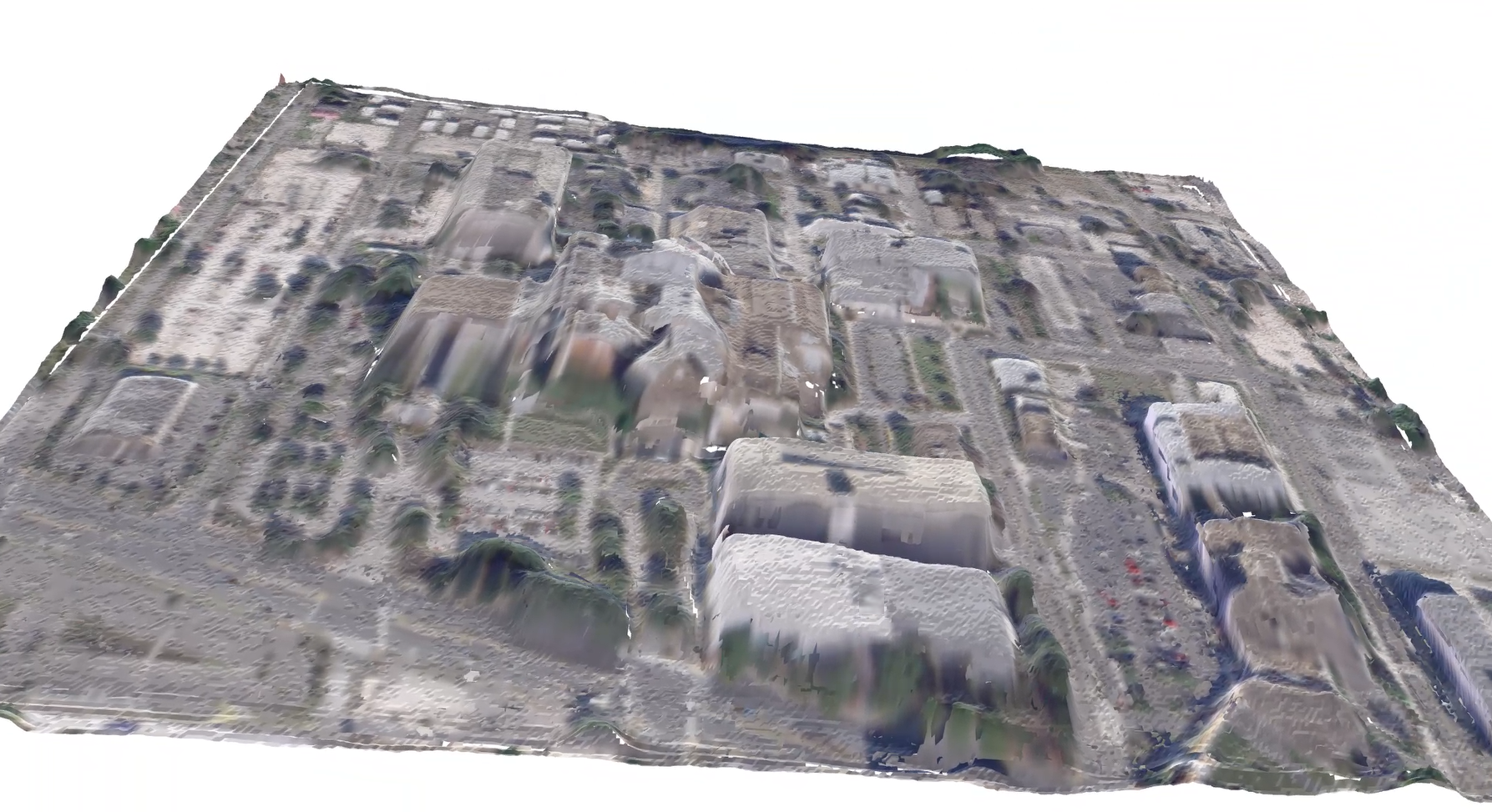
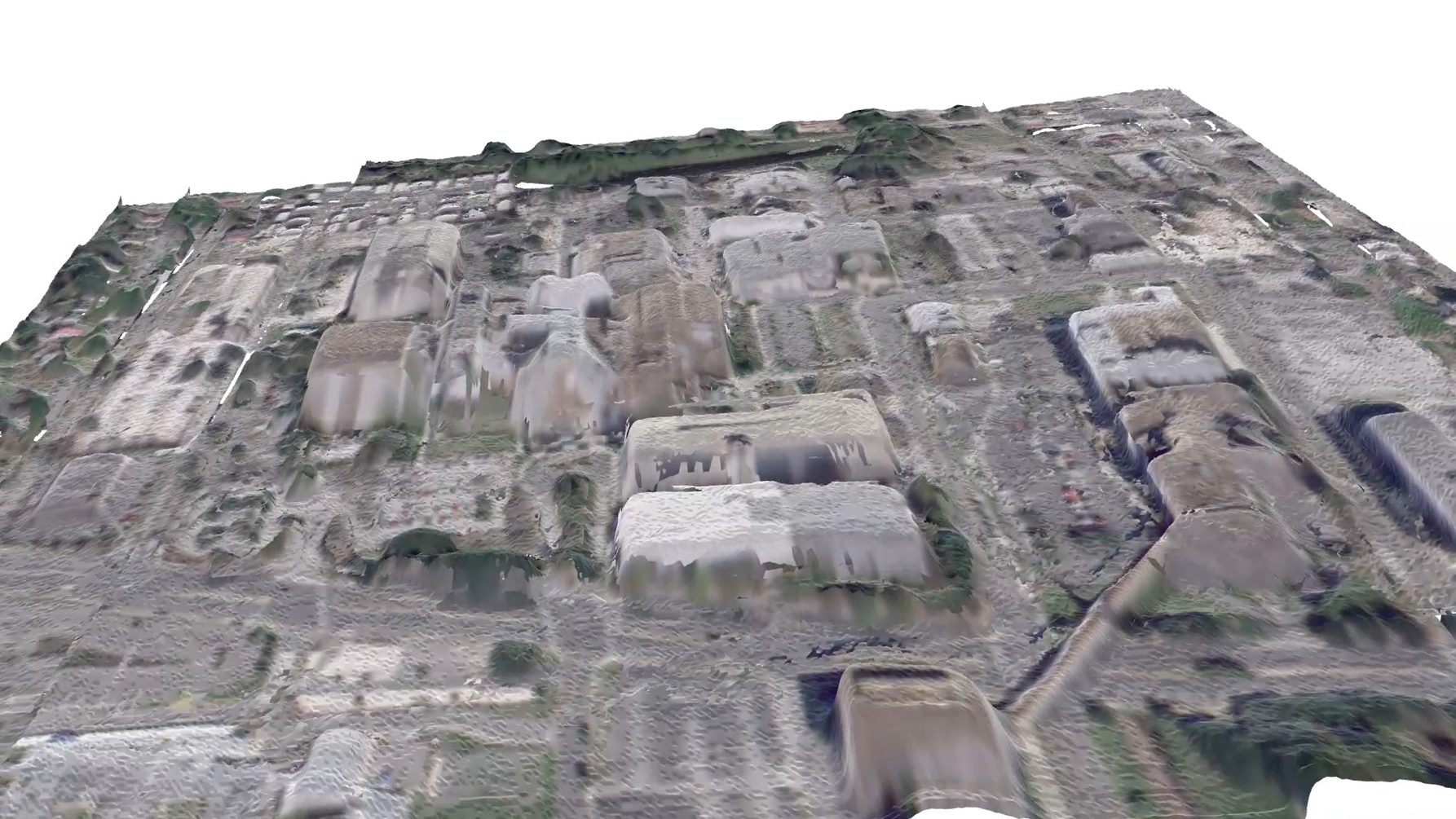
Figure 7. Most spread (right) recovered more area, has less gaps, and more defined edges in building geometry than least spread (left).

Figure 8. Gap and poor geometry visualization for the least-spread (left) and it mostly fixed in most-spread (right).

Key Insights:

DUSt3R demonstrates robust reconstruction performance even with a limited number of views.
Brute forcing training by adding additional views does not necessarily increase model quality.
Strategic view selection provides improvements in reconstruction quality when compared to suboptimal view configurations when there is sufficient image overlap, particularly in areas of complex geometry like tall buildings.
In our satellite imagery application, where perspective variations can be substantial, strategic view selection becomes particularly valuable for achieving quality reconstructions.

5. Conclusion

In this paper, we investigated the feasibility of 3D reconstruction from sparse satellite imagery, comparing three distinct approaches: 3D Gaussian Splatting, VGGT with bundle adjustment optimization, and DUSt3R. Our experiments demonstrate that meaningful 3D reconstruction from limited satellite imagery can be achieved with appropriate techniques. We found that while standard 3DGS struggles with the sparse viewpoints and similar camera properties of satellite imagery, VGGT with bundle adjustment produces compelling results through its multi-stage optimization process that effectively handles confidence-weighted point selection.DUSt3R offers the most reliable reconstructions when paired with our camera spread optimization technique, which mitigates the combinatorial explosion in training time while improving reconstruction quality. Additionally, our camera selection methodology based on Fisher information theory enhances reconstruction quality across all methods, particularly for complex structures. These findings suggest practical applications for rapid 3D reconstruction from satellite imagery in scenarios where data collection is limited or time-sensitive, such as disaster response or remote terrain analysis.